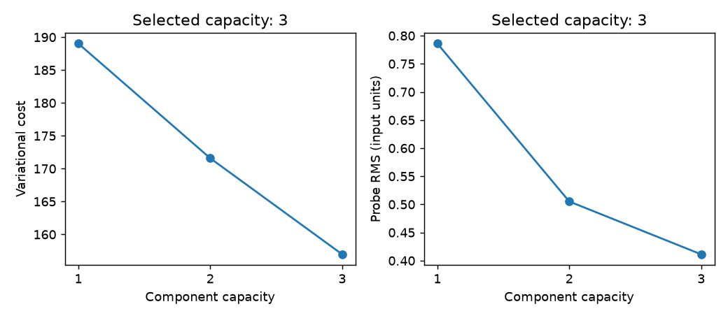
Cost versus probe RMS

Both criteria use the same held-out cells and positive capacities. Rank zero has no variational cost. Cost and probe RMS have different units and are plotted on separate axes; these short sweeps do not qualify a selection policy.

These synthetic examples run at most eight fit iterations. They demonstrate API behavior; they do not establish posterior convergence, calibration or a recommended capacity.

This example uses the 0.5 API with the plot extra. From a matching source checkout, install python -m pip install '.[plot]', then run python scripts/gallery_selection.py --output-dir outputs. The downloaded source can also run directly against that installed 0.5 build.

Download this standalone source.

Output

{
  "selected_capacity": {
    "cost": 3,
    "prms": 3
  },
  "common_probe_cells": 5,
  "records": [
    {
      "k": 1,
      "cost": 189.03411532522344,
      "prms": 0.7860246936967983
    },
    {
      "k": 2,
      "cost": 171.5860896877125,
      "prms": 0.5051694580924303
    },
    {
      "k": 3,
      "cost": 156.97196014329776,
      "prms": 0.41122587681948575
    }
  ]
}

Candidate records

k	cost	prms
1	189.034	0.786025
2	171.586	0.505169
3	156.972	0.411226

Executed source

"""Compare cost and probe-RMS selection on the same held-out observations."""

import argparse
import json
from pathlib import Path

import matplotlib.pyplot as plt
import numpy as np

from vbpca_py import SelectionConfig, select_n_components


def run_example(output_dir):
    rng = np.random.default_rng(25)
    x = rng.normal(size=(24, 2)) @ rng.normal(size=(2, 5))
    x += 0.3 * rng.normal(size=x.shape)
    x[0, 0] = np.nan
    probe = np.full_like(x, np.nan)
    for row, column in [(2, 0), (5, 1), (8, 2), (11, 3), (14, 4)]:
        probe[row, column] = x[row, column]
    options = {
        "maxiters": 8,
        "niter_broadprior": 0,
        "random_state": 25,
        "runtime_tuning": "off",
        "num_cpu": 1,
        "verbose": 0,
    }
    selected, traces = {}, {}
    for metric in ["cost", "prms"]:
        chosen, _, trace, _ = select_n_components(
            x,
            xprobe=probe,
            components=[1, 2, 3],
            config=SelectionConfig(metric=metric),
            **options,
        )
        selected[metric] = chosen
        traces[metric] = trace
    fig, axes = plt.subplots(1, 2, figsize=(8, 3.5))
    for ax, metric, label in zip(
        axes,
        ["cost", "prms"],
        ["Variational cost", "Probe RMS (input units)"],
        strict=True,
    ):
        trace = traces[metric]
        ax.plot(
            [record["k"] for record in trace],
            [record[metric] for record in trace],
            "o-",
        )
        ax.set(
            xlabel="Component capacity",
            ylabel=label,
            xticks=[1, 2, 3],
            title=f"Selected capacity: {selected[metric]}",
        )
    fig.tight_layout()
    output_dir.mkdir(parents=True, exist_ok=True)
    fig.savefig(output_dir / "selection.png", dpi=130)
    plt.close(fig)
    summary = {
        "selected_capacity": selected,
        "common_probe_cells": int(np.isfinite(probe).sum()),
        "records": [
            {key: record[key] for key in ["k", "cost", "prms"]}
            for record in traces["cost"]
        ],
    }
    (output_dir / "summary.json").write_text(json.dumps(summary, indent=2) + "\n")
    print(json.dumps(summary, indent=2))


if __name__ == "__main__":
    parser = argparse.ArgumentParser(description=__doc__)
    parser.add_argument("--output-dir", type=Path, required=True)
    run_example(parser.parse_args().output_dir)